1 Probability Theory Primer

Author

Aribah

Modified

December 23, 2024

Hello, Students!

Students, write your notes in the corresponding .qmd files under the students/ folder. The Editor will then merge everything into one cohesive notes.

BTW, for more callout blocks, look here: https://quarto.org/docs/authoring/callouts.html

Lorem ipsum dolor sit amet, consectetur adipiscing elit. Duis sagittis posuere ligula sit amet lacinia. Duis dignissim pellentesque magna, rhoncus congue sapien finibus mollis. Ut eu sem laoreet, vehicula ipsum in, convallis erat. Vestibulum magna sem, blandit pulvinar augue sit amet, auctor malesuada sapien. Nullam faucibus leo eget eros hendrerit, non laoreet ipsum lacinia. Curabitur cursus diam elit, non tempus ante volutpat a. Quisque hendrerit blandit purus non fringilla. Integer sit amet elit viverra ante dapibus semper. Vestibulum viverra rutrum enim, at luctus enim posuere eu. Orci varius natoque penatibus et magnis dis parturient montes, nascetur ridiculus mus.

Example 1.1 \[ y \sim \text{N}(\mu, \sigma^2) \]

Check out https://quarto.org/docs/authoring/cross-references.html#theorems-and-proofs for more div types (like theorem, lemmas, proofs, etc.).

Figure 1.1 shows an image.

Write R code like this:

```{r}
1 + 1
```

Which will be rendered as:

Code

1 + 1

[1] 2

Tip

Feel free to rearrange the sections however you wish. Below, you will find some extra bits that you may want to include as part of your notes, or just leave them as the appendix.

1.1 Algebras of sets

This is the mathematical structure that allows us to observe and measure random events. Logically,

If an event \(A\) can be observed, then its complement can be too. I.e. \(A \in {\mathcal F}\Rightarrow A^c \in {\mathcal F}\).
At least one outcome can be observed, i.e. \(\Omega \in {\mathcal F}\).
If two or more events are observed, then at least one of them (or both) can be observed, i.e. \[ A,B \in {\mathcal F}\Rightarrow A \cup B \in {\mathcal F} \]

If 1–3 holds, then \({\mathcal F}\) is said to be an algebra over \(\Omega\). In addition, if you can “add” up infinitely many countable things, \({\mathcal F}\) is called a \(\sigma\)-algebra. \[ A_1,A_2,\dots \in{\mathcal F}\Rightarrow \bigcup_{i=1}^\infty A_i \in {\mathcal F} \]

1.2 Why \(\sigma\)-algebra?

In probability theory and statistics, an experiment (or trial) is a procedure that can be repeated and has a well-defined set of possible outcomes (known as the sample space \(\Omega\)). Events are thought of as being subsets of \(\Omega\), while probabilities are merely a mapping from some event space \(\mathcal F\) to \([0,1]\).

To make this idea concrete, for the die roll example, \(\Omega=\{1,\dots,6\}\), while an event could be \(E=\{2,4,6\}\subset \Omega\) (getting an even number). The probability of the event \(E\) occurring is \(\operatorname{P}(E)=\frac{1}{2}\)–so it indeed behaves like a function, taking input some event and spitting out a number between 0 and 1.

Note here that \(\mathcal F\) is not \(\Omega\)–it has to be bigger than \(\Omega\) as we’re not just interested in singleton outcomes. A good starting point would be \(\mathcal F = \mathcal P(\Omega)\), the set of all subsets of \(\Omega\), which should contain all possible events constructed from the set of outcomes.

1.2.1 Rules of probability

Having abstracted the notion of \(\Omega\) and \(\mathcal F\), we should also define some rules that the probability function \(\operatorname{P}:\mathcal P(\Omega)\to[0,1]\) must follow. Let us list down a few:

\(\operatorname{P}(E) \geq 0, \forall E\);
\(\operatorname{P}(\varnothing)=0\) and \(\operatorname{P}(\Omega) = 1\);¹
If \(E_1 \cap E_2 = \varnothing\), then \(\operatorname{P}(E_1 \cup E_2)=\operatorname{P}(E_1) + \operatorname{P}(E_2)\); and
If \(E_1, E_2,\dots\) are mutually disjoint events, then \(\operatorname{P}\Big(\bigcup_{i=1}^\infty E_i \Big) = \sum_{i=1}^\infty \operatorname{P}(E_i)\).

Indeed, these are quite logical impositions that ensure we don’t end up with nonsensical probabilities. For instance, by ii. and iii., modelling a (biased) coin toss by \(\operatorname{P}(H)=0.7\) necessitates \(\operatorname{P}(T)=0.3\) and not anything else, e.g. \(\operatorname{P}(T)=0.5\).

1.2.2 The need for measure theory

We’ve managed to come up with probability rules so far without the need for measure theory, so what’s the problem? The problem is that in the way that we’ve described it, this is actually too much to ask! There will be instances where this whole framework fails and we can’t assign probabilities properly, especially when we need it the most.

Consider that, with all these demands, we can’t even define the uniform random variable on \(\Omega=[0,1]\)! That is, no mapping \(\operatorname{P}:\mathcal P([0,1])\to[0,1]\) exists such that \(\operatorname{P}([a,b])=b-a\) for \(0\leq a \leq b \leq 1\) which satisfies all of the rules i. to iv. listed above. For a proof, see the appendix. Evidently some concession has to be made (which one?), and the probability map must be constructed more carefully. The answer lies in measure theory.

1.3 An unmeasurable set

As mentioned, we are unable to define a uniform probability measure on the unit interval, given by \[ \operatorname{P}([a,b]) = b-a \] that satisfies all the probability rules listed in i. to iv. earlier. On the face of it, all the rules themselves are satisfied: \(\operatorname{P}(\Omega)=\operatorname{P}([0,1])=1\), \(\operatorname{P}(\varnothing)=\operatorname{P}([a,a])=0\) (for any \(a\in[0,1]\)), and certainly probabilities of disjoint subsets of \([0,1]\) are just the sum of the lengths of the intervals.

These are all great properties to have, so we must concede instead on the domain of the probability function, i.e. the event space. The proof of the proposition below in instructive, in that it illustrates the existence of a “non-measurable” set. That is, there are such events (subsets in \([0,1]\)) for which we are unable to assign probabilities to.

Proposition 1.1 There does not exist a definition of \(\operatorname{P}:\mathcal P([0,1])\to[0,1]\) satisfying \(\operatorname{P}([a,b])=b-a\) and i. to iv. (as listed earlier).

Proof. All we need to show is the existence of one such subset of \([0,1]\) whose measure is undefined. The set we are about to construct is called the Vitali set², after Giuseppe Vitali who described it in 1905.

Before proceeding, we introduce some notation. For a uniform measure on \([0,1]\), one expects that the measure of some subset \(A \subseteq [0,1]\) to be unaffected by “shifting” (with wrap-around) of that subset by some fixed amount \(r\in[0,1]\). Define the \(r\)-shift of \(A\subseteq [0,1]\) by \[ A \oplus r := \left\{ a + r \mid a \in A, a+r \leq 1 \right\} \cup \left\{ a + r - 1 \mid a \in A, a+r > 1 \right\}. \] Then we should have \[ \operatorname{P}(A \oplus r) = \operatorname{P}(A). \] For example, \(\operatorname{P}([0.7, 0.9] \oplus 0.2) = \operatorname{P}([0.9,1] \cup [0,0.1]) = 0.2\).

Now, define an equivalence relation on \([0,1]\) by the following: \[x\sim y \Rightarrow y-x \in \mathbb Q\] That is, two real numbers \(x\) and \(y\) are deemed to be similar if their difference is a rational number. The intent is to segregate all the real numbers \(x\in[0,1]\) by this equivalence relation, and collect them into groups called equivalence classes, denoted by \([x]\). Here, \([x]\) is the set \(\{y \in [0,1] \mid x \sim y\}.\) For instance,

The equivalence class of \(0\) is the set of real numbers \(x\) such that \(x \sim 0\), i.e. \([0] = \{y \in [0,1] \mid y-0\in\mathbb Q \}\), which is the set of all rational numbers in \([0,1]\).
The equivalence class of an irrational number \(z_1\in[0,1]\) is clearly not in \([0]\), thus would represent a different equivalence class \([z_1]=\{y \in [0,1] \mid y-z_1 \in \mathbb Q \}\).
Yet another irrational number \(z_2\not\in [z_1]\) would exist, i.e. a number \(z_2\in[0,1]\) such that \(z_2-z_1 \not\in\mathbb Q\), and thus would represent a different equivalence class \([z_2]\).
And so on…

The equivalence classes may therefore be represented by \([0],[z_1],[z_2],\dots\) where \(z_i\) are all irrational numbers that differ by an irrational number, and there are uncountably many such numbers, and therefore classes.

Construct the Vitali set \(V\) as follows: Take precisely one element from each equivalent class, and put it in \(V\). As a remark, such a \(V\) must surely exist by the Axiom of Choice³.

Consider now the union of shifted Vitali sets by some rational value \(r\in[0,1]\), \[ \bigcup_{r} (V \oplus r) \] As a reminder, the set of rational numbers is countably infinite⁴. We make two observations:

The equivalence relation partitions the interval \([0,1]\) into a disjoint union of equivalence classes. In other words, the sets \((V \oplus r)\) and \((V \oplus s)\) are disjoint for any rationals \(r\neq s\), such that \(r,s\in[0,1]\). If they were not disjoint, this would mean that there exists some \(x,y\in[0,1]\) with \(x+r\in(V \oplus r)\) and \(y+s\in (V \oplus s)\) such that \(x+r=y+s\). But then this means that \(x-y=s-r\in\mathbb Q\) so \(x\) and \(y\) are in the same equivalent class, and this is a contradiction. Importantly, \[\begin{equation}\label{eq:contr1} \operatorname{P}\left(\bigcup_{r} (V \oplus r)\right) = \sum_r \operatorname{P}(V \oplus r) = \sum_r \operatorname{P}(V) \end{equation}\]
Every point in \([0,1]\) is contained in the union \(\bigcup_{r} (V \oplus r)\). To see this, fix a point \(x\) in \([0,1]\). Note that this point belongs to some equivalent class of \(x\), and in this equivalence class there exists some point \(\alpha\) which belongs to \(V\) as well by construction. Hence, \(\alpha \sim x\), and thus \(x-\alpha=r\in\mathbb Q\), implying that \(x\) is a point in the Vitali set \(V\) shifted by \(r\). Therefore, \[[0,1] \subseteq \bigcup_{r} (V \oplus r).\] and we may write \[1 = \operatorname{P}([0,1]) \leq \operatorname{P}\left(\bigcup_{r} (V \oplus r)\right)\leq 1,\] since the measure of any set contained in another must have smaller or equal measure (a relation implied by property iii.⁵) as well as all probabilities are less than equal to 1⁶. We see that \[\begin{equation}\label{eq:contr2} \operatorname{P}\left(\bigcup_{r} (V \oplus r)\right) = 1. \end{equation}\]

Equating \(\eqref{eq:contr1}\) and \(\eqref{eq:contr2}\) together, we find a contradiction: A countably infinite sum of a constant value can only equal \(0\), \(+\infty\) or \(-\infty\), but never 1.

1.4 Conditional probability

The latest estimate puts the proportion of geology students at FOS to be 5%. A randomly selected student from FOS, Nafeesah, is described by her peers as someone who loves the outdoors and gets overly excited when shown something that is related to rocks.

Which statement is more likely?

Nafeesah is undertaking a BSc Geology programme.
Nafeesah is not undertaking a BSc Geology programme.

Let

\(E\) be the ‘evidence’
\(G\) be the event that a student takes Geology

Then \[ \operatorname{P}(G|E) = \frac{\operatorname{P}(E|G)\operatorname{P}(G)}{\operatorname{P}(E)} \approx \frac{0.05}{\operatorname{P}(E)} \]

Code

x <- seq(1e-10, 1, length = 100)
plot_df <- tibble(
  x = x,
  y = 0.05 / x
)

ggplot(plot_df, aes(x, y)) +
  geom_line() +
  geom_segment(x = -Inf, xend = 0.05 / 0.5, y = 0.5,yend = 0.5,
               linetype = "dashed", col = "red3") +
  geom_segment(x = 0.05 / 0.5, xend = 0.05 / 0.5, y = 0.5, yend = -Inf,
               linetype = "dashed", col = "red3") +
  scale_y_continuous(limits = c(0, 1)) +
  scale_x_continuous(breaks = seq(0, 1, by = 0.2)) +
  labs(x = "P(E)", y = "P(G|E)")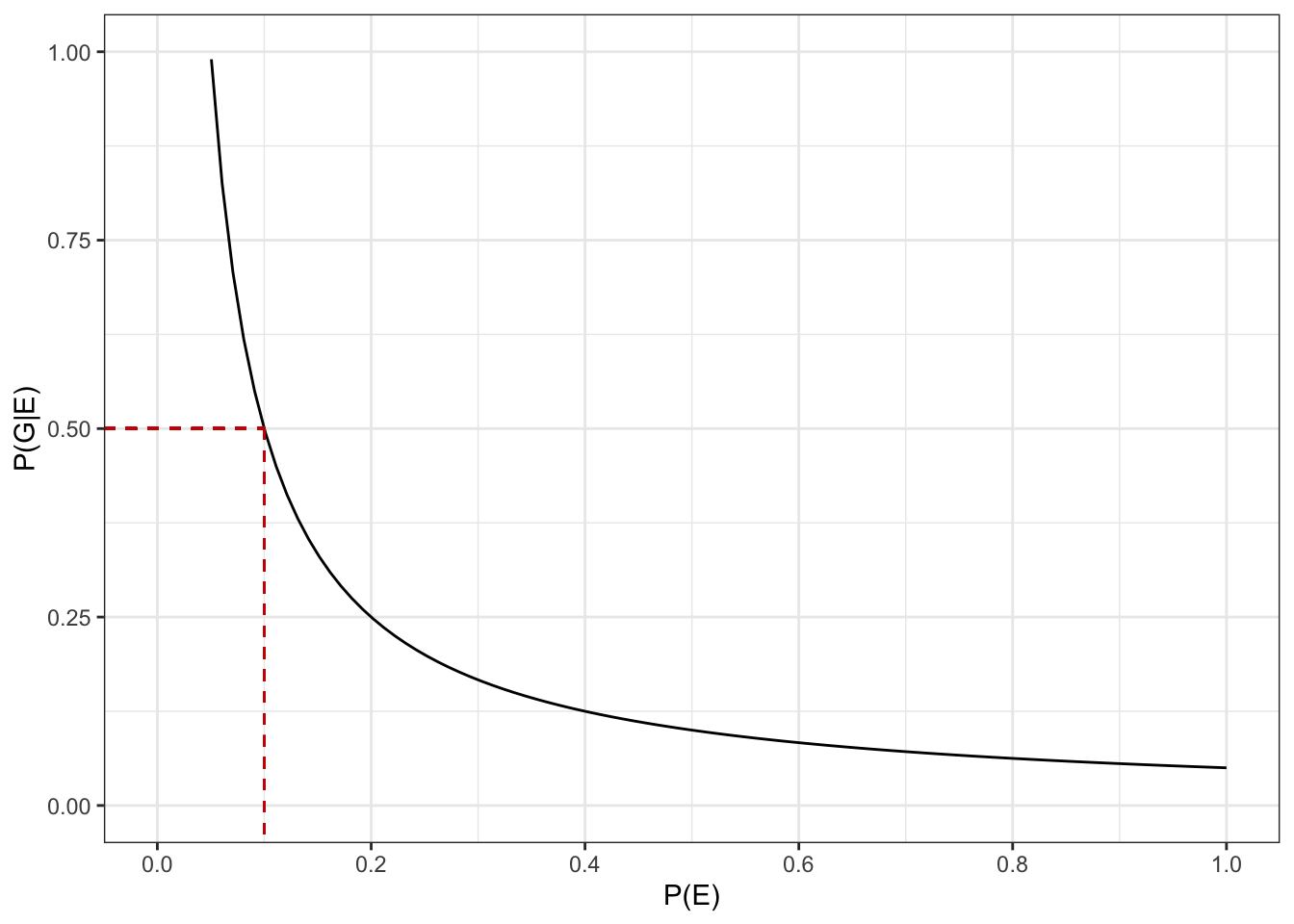

1.5 Bayesian statistics

Sometime between 1746 and 1749, Rev. Thomas Bayes conducted this experiment.

Imagine a square, flat table. You throw a marker (e.g. a coin) but do not know where it lands. You ask an assistant to randomly throw a ball on the table. The assistant informs you whether it stopped to the left or right from the first ball. How to use this information to better estimate where your marker landed?

The Bayesian principle is about updating beliefs.

Let \(X \in [0,1]\) be the location of the ball on a horizontal axis.
Before any new information, any position \(X\) is possible, say \(X\sim\mathop{\mathrm{Unif}}(0,1)\).
Let \(Y\) be the number of times the assistant’s ball landed left of the marker after \(n\) throws. Then \(Y|X \sim \mathop{\mathrm{Bin}}(n,X)\).
What we want is information regarding \(X|Y\), which is obtained using Bayes Theorem \[ \operatorname{P}(X\in x|Y=y) = \frac{\operatorname{P}(Y=y|X\in x)\operatorname{P}(X\in x)}{\operatorname{P}(Y=y)} \]

Code

# https://dosreislab.github.io/2019/01/27/ballntable.html
set.seed(123)
n <- 15
xy <- runif(2) # position of coin after intial throw
xy.2 <- matrix(runif(2 * n), ncol=2) # additional n throws of the ball

pos <- numeric(2)
pos[1] <- sum(xy.2[,1] < xy[1])
pos[2] <- sum(xy.2[,2] < xy[2])

jointf <- function(pos = pos, n = n, N=100) {
  a <- pos[1]; b <- pos[2]
  x <- y <- seq(from=0, to=1, len=N)
  xf <- x^a * (1-x)^(n-a)
  yf <- y^b * (1-y)^(n-b)
  z <- xf %o% yf
}

Cf <- function(x, y, n) {
  ( factorial(n+1) )^2 /
  ( factorial(x) * factorial(n-x) * factorial(y) * factorial(n-y) )
}

z <- jointf(pos, n) * Cf(pos[1], pos[2], n)

as.data.frame(z) %>%
  `colnames<-`(1:100 / 100) %>%
  rownames_to_column() %>%
  gather(key, value, -rowname) %>%
  mutate(rowname = as.numeric(rowname) / 100,
         key = as.numeric(key)) %>%
  ggplot(aes(rowname, key, z = value)) +
  geom_contour() +
  geom_point(x = xy[1], y = xy[2]) +
  lims(x = c(0, 1), y = c(0, 1))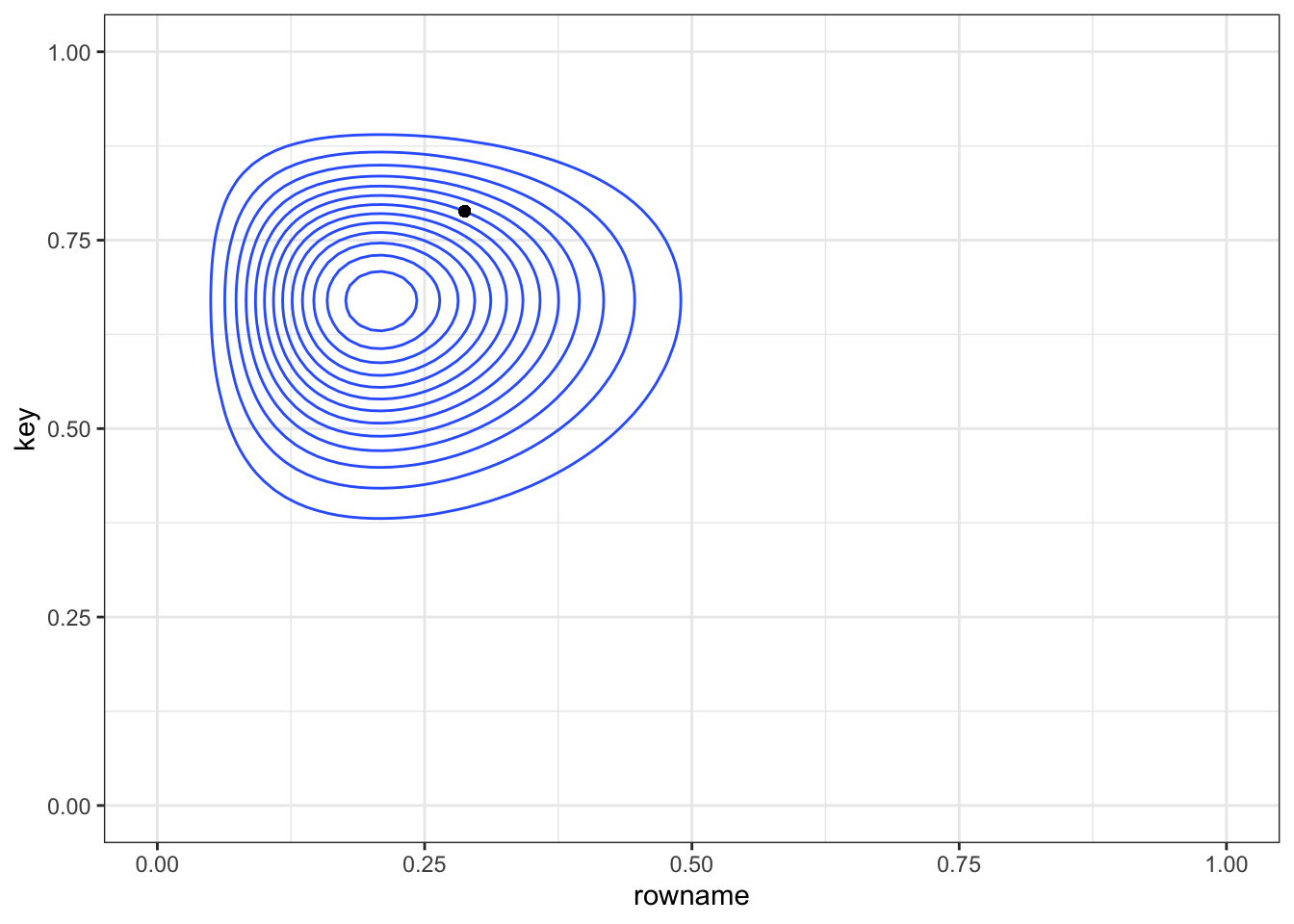

1.6 Probability integral transform

Theorem 1.1 Let \(X\) have continuous cdf \(F_X(x)\) and define the random variable \(Y\) as \(Y=F_X(X)\). Then \(Y\) is uniformly distributed on \((0,1)\), that is \(f_Y(y)=1 \ \forall y\in[0,1]\) with \(\operatorname{P}(Y\leq y)=y\).

Proof. \[\begin{align*} \operatorname{P}(Y \leq y) &= \operatorname{P}(F_X(X) \leq y) \\ &= \operatorname{P}\big(X \leq F_X^{-1}(y)\big) \\ &= F_X\big(F_X^{-1}(y) \big) = y. \end{align*}\]

The PIT is a special kind of transformation, useful for various statistical purposes. Suppose we wish to generate \(X\sim F_X\)–this is done via \(X=F_X^{-1}(U)\) where \(U\sim\mathop{\mathrm{Unif}}(0,1)\).

\(\varnothing = \{ \}\) is the empty set.↩︎
https://en.wikipedia.org/wiki/Vitali_set↩︎
Given a collection of non-empty sets, it is always possible to construct a new set by taking one element from each set in the original collection. See https://brilliant.org/wiki/axiom-of-choice/↩︎
https://www.homeschoolmath.net/teaching/rational-numbers-countable.php↩︎
Let \(A\) and \(B\) be such that \(A \subseteq B\). Then we may write \(B = A \cup (B\setminus A)\) where the sets \(A\) and \(B \setminus A\) are disjoint. Hence, \(\operatorname{P}(B)=\operatorname{P}(A)+\operatorname{P}(B \setminus A)\), and since probabilities are non-negative, we have that \(\operatorname{P}(B)\geq \operatorname{P}(A)\).↩︎
For any \(A\), \(\operatorname{P}(\Omega)=\operatorname{P}(A \cup A^c) = \operatorname{P}(A) + \operatorname{P}(A^c) = 1\), so \(\operatorname{P}(A)\leq 1\).↩︎