Code
n <- 10
theta_pp <- 0.8  # PRETEND YOU DON'T KNOW THIS

X <- rbinom(n = n, size = 1, prob = theta_pp)
X
[1] 1 1 1 1 1 0 0 1 1 0These are the notes for SM-4331 Advanced Statistics.
Statistics is a scientific subject on collecting and analysing data.
Collecting means designing experiments, designing questionnaires, designing sampling schemes, administration of data collection.
Analysing means modelling, estimation, testing, forecasting.

Statistics is an application-oriented mathematical subject; it is particularly useful or helpful in answering questions such as:
There are three aspects to learning statistics:
In this course, there is an emphasis on the theory aspect of statistics.
Students who analyze data, or who aspire to develop new methods for analyzing data, should be well grounded in basic probability and mathematical statistics. Using fancy tools like neural nets, boosting, and support vector machines without understanding basic statistics is like doing brain surgery before knowing how to use a band-aid.
—Larry Wasserman (in All of Statistics)
In Brunei, boba tea is a sensation, with countless shops vying for the title of the “best” through customer satisfaction ratings. Tapioca Treasure, one of the crowd favorites, boasts an impressive 4.3 out of 5-star rating—based on a simple question: Do you like their bubble tea?

Intrigued, you and a friend decide to visit and sample their offerings. This raises some interesting probability-based questions:
Exercise 1.1
[Of course, these questions involve certain assumptions, which we’ll discuss in a bit.]
Solution 1.1. Let \(X\) represent whether a person likes the bubble tea at Tapioca Treasure. We may write \[ X = \begin{cases} 1 & \text{likes tea} \\ 0 & \text{does not like tea} \\ \end{cases} \] which is a convenient way of “coding” the qualitative response of like / do not like into numbers (1/0). Suppose that \(X\) is a random variable, then we may also write \[ \operatorname{P}(X=1) := \theta = 0.86, \] based on the shop’s 4.3/5 star rating, interpreted as an 86% likelihood of liking the bubble tea. Since \(X\) is a binary random variable (i.e. takes only two outcomes), \(X\) is said to follow a Bernoulli distribution1.
Since \(X \sim \text{Bernoulli}(\theta)\), the probability that you like the bubble tea is simply: \[ P(X = 1) = \theta = 0.86. \]
Let \(Y\) denote whether you or your friend like the bubble tea. Assume the two events are independent. The probability that at least one of you likes the bubble tea is given by: \[\begin{align*} \operatorname{P}(Y \geq 1) &= 1 - P(\text{neither likes it}) \\ &= 1 - P(X_1 = 0)P(X_2 = 0), \end{align*}\] where \(X_1\) and \(X_2\) represent your and your friend’s preferences, respectively. Substituting the values: \[\begin{align*} P(Y \geq 1) &= 1 - (1 - \theta)(1 - \theta) \\ &= 1 - (1 - 0.86)^2 \\ &= 1 - 0.14^2 \\ &= 1 - 0.0196 \\ &= 0.9804. \end{align*}\] Thus, there is approximately a 98.04% chance that at least one of you will like the bubble tea.
If you invite your entire family of size \(n\), the number of people who like the bubble tea \(S\) is known to follow a Binomial distribution: \[ S \sim \text{Binomial}(n, \theta). \] Using properties of the Binomial distribution, the expected value of a Binomial random variable is given by: \[ E(S) = n\theta. \] Substituting the values: \[ E(S) = 0.86n. \]
In part (b) above, we came to the solution by assuming that you and your friend have the same probability of liking the tea. In other words, your preferences are independent of each other2.
In fact, for the binomial distribution, this same assumption must be met for all your family members.
Suppose you’re hired by a new boba tea shop, Pearl Paradise, to determine whether their signature drink is as good as their rival’s, Tapioca Treasure.


The questions we have to answer are:
Exercise 1.2
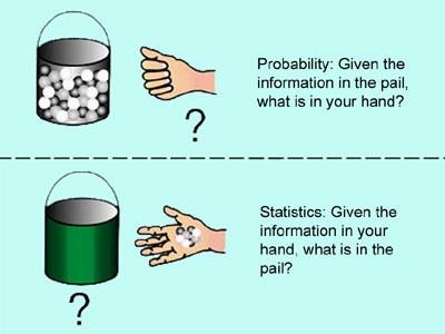
Notice how these questions are fundamentally different from the previous questions. Previous calculations are “straightforward” if you know probabilities and distribution theory, since the \(\theta\) value is given. Here, you’re dealing with the fact that the \(\theta\) values is unknown, and somehow is the focus of attention.
The other thing you might realise is that there is no way of answering the questions without having data points to infer from. This is the difference between statistics and probability. The above three questions implicitly describe the three main activities concerning statistical inference: 1. Point estimation; 2. Hypothesis testing; and 3. Interval estimation.
For now, let us assume that we may collect some data, to at least answer the first part (a). You conduct a survey of 10 random individuals, and ask them the question “Do you like the bubble tea from Pearl Paradise?”. Here are the responses to the survey:
n <- 10
theta_pp <- 0.8 # PRETEND YOU DON'T KNOW THIS
X <- rbinom(n = n, size = 1, prob = theta_pp)
X [1] 1 1 1 1 1 0 0 1 1 0Let us denote \(X_i\) to be the response for individual \(i\) to the survey. So in the above, \(X_1 = 1\), \(X_2 = 1\), and so on. The assumption we make here, similar to the probability question above, is that \(X_i\sim\text{Bern}(\theta)\) independently. Let’s now work through the solutions:
Solution 1.2.
We often denote the estimate of \(\theta\) by its hat version, so we often write \[ \hat\theta = 0.7. \]
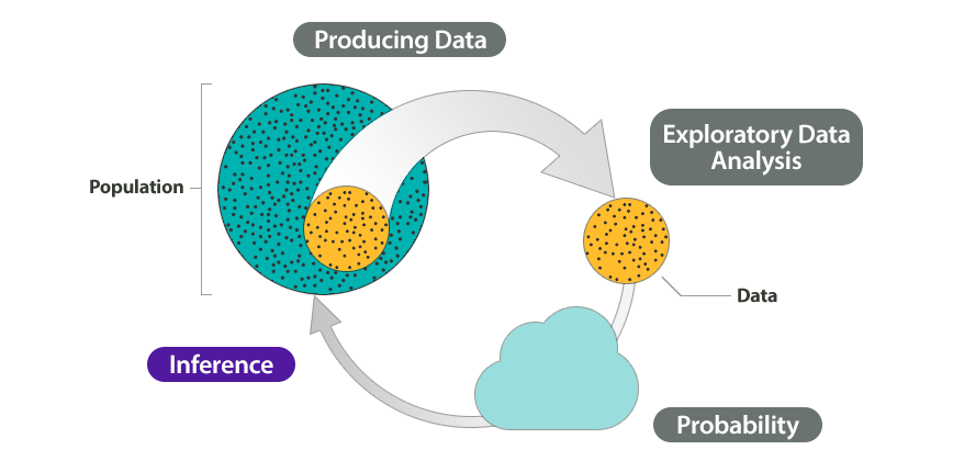
I am sure you notice, that the estimate \(\hat\theta\) will depend on who you ask in the survey. In the context of Pearl Paradise, the population represents all potential customers who could provide their opinion about the boba tea, while the sample refers to the subset of individuals surveyed.
Consider a random sample of size \(n\) (in the example above, \(n=10\)): \[ \mathcal S = \{X_1,\dots,X_n\}. \] Here \(X_i\) are concrete numbers or data regarding the population which is pertinent to answer your statistical question. In statistical inference, we use the sample data to estimate characteristics of the population, such as the proportion of customers who like Pearl Paradise’s boba tea. Since it is often impractical to survey the entire population, we rely on the sample to draw conclusions, recognizing that there is uncertainty due to sampling variability.
Of course, a lot of things can influence this, such as demographics, time period, circumstances, non-response rates, etc. – and there’s a lot of work to ensure “representativeness” of a sample, but our course does not deal with this.
But even if all things perfect, there is inherent randomness due to sampling itself. We can simulate this by repeatedly conducting the survey of 10 people. Here are the results:
B <- 20  # number of repeated surveys
res <- list()
for (i in 1:B) {
  res[[i]] <- rbinom(n = n, size = 1, prob = theta_pp)
}

tab <-
  tibble(
    survey = 1:B,
    X = res
  ) |>
  mutate(
    theta_hat = sapply(X, mean),
    X = sapply(X, \(x) paste0(x, collapse = ","))
  )

gt(tab) |>
  fmt_markdown() |>
  cols_label(
    survey ~ "Survey no.",
    theta_hat ~ gt::md("$\\hat\\theta$")
  ) |>
tab_options(quarto.disable_processing = TRUE)| Survey no. | X | \(\hat\theta\) |
|---|---|---|
| 1 | 0,1,1,1,1,1,1,1,1,1 | 0.9 |
| 2 | 1,1,1,0,1,1,1,1,1,0 | 0.8 |
| 3 | 1,1,1,1,1,1,1,1,1,0 | 0.9 |
| 4 | 1,1,1,1,1,0,1,1,1,1 | 0.9 |
| 5 | 1,1,0,1,0,1,1,1,1,1 | 0.8 |
| 6 | 1,1,1,1,0,1,1,1,1,1 | 0.9 |
| 7 | 1,1,1,1,1,1,1,1,1,0 | 0.9 |
| 8 | 0,1,1,1,1,1,1,1,1,1 | 0.9 |
| 9 | 0,1,1,1,1,0,1,1,0,1 | 0.7 |
| 10 | 1,1,1,1,1,0,1,1,1,1 | 0.9 |
| 11 | 1,1,1,1,1,1,0,1,0,1 | 0.8 |
| 12 | 1,1,0,1,0,0,1,1,0,0 | 0.5 |
| 13 | 1,1,1,0,1,1,1,1,1,0 | 0.8 |
| 14 | 1,1,1,1,1,0,1,1,1,1 | 0.9 |
| 15 | 0,1,1,1,1,1,1,1,1,1 | 0.9 |
| 16 | 1,0,0,1,1,1,1,1,1,1 | 0.8 |
| 17 | 1,1,0,1,1,1,1,1,1,1 | 0.9 |
| 18 | 0,1,1,1,0,1,0,1,1,0 | 0.6 |
| 19 | 1,1,1,1,1,1,1,1,1,0 | 0.9 |
| 20 | 1,1,1,0,1,0,1,1,1,1 | 0.8 |
Suppose we conducted more and more of the surveys, we could even get more information regarding the variability of the estimator. Ideally, we could even plot a histogram to show the distribution of the estimator.
B <- 100000  # number of repeated surveys
theta_hats <- c()
for (i in 1:B) {
  theta_hats[i] <- mean(rbinom(n = n, size = 1, prob = theta_pp))
}

tibble(
  theta_hat = theta_hats
) |>
  ggplot(aes(x = theta_hat)) +
  geom_histogram(fill = "lightblue", col = "black", binwidth = 0.05) +
  scale_x_continuous(breaks = seq(0, 1, by = 0.1))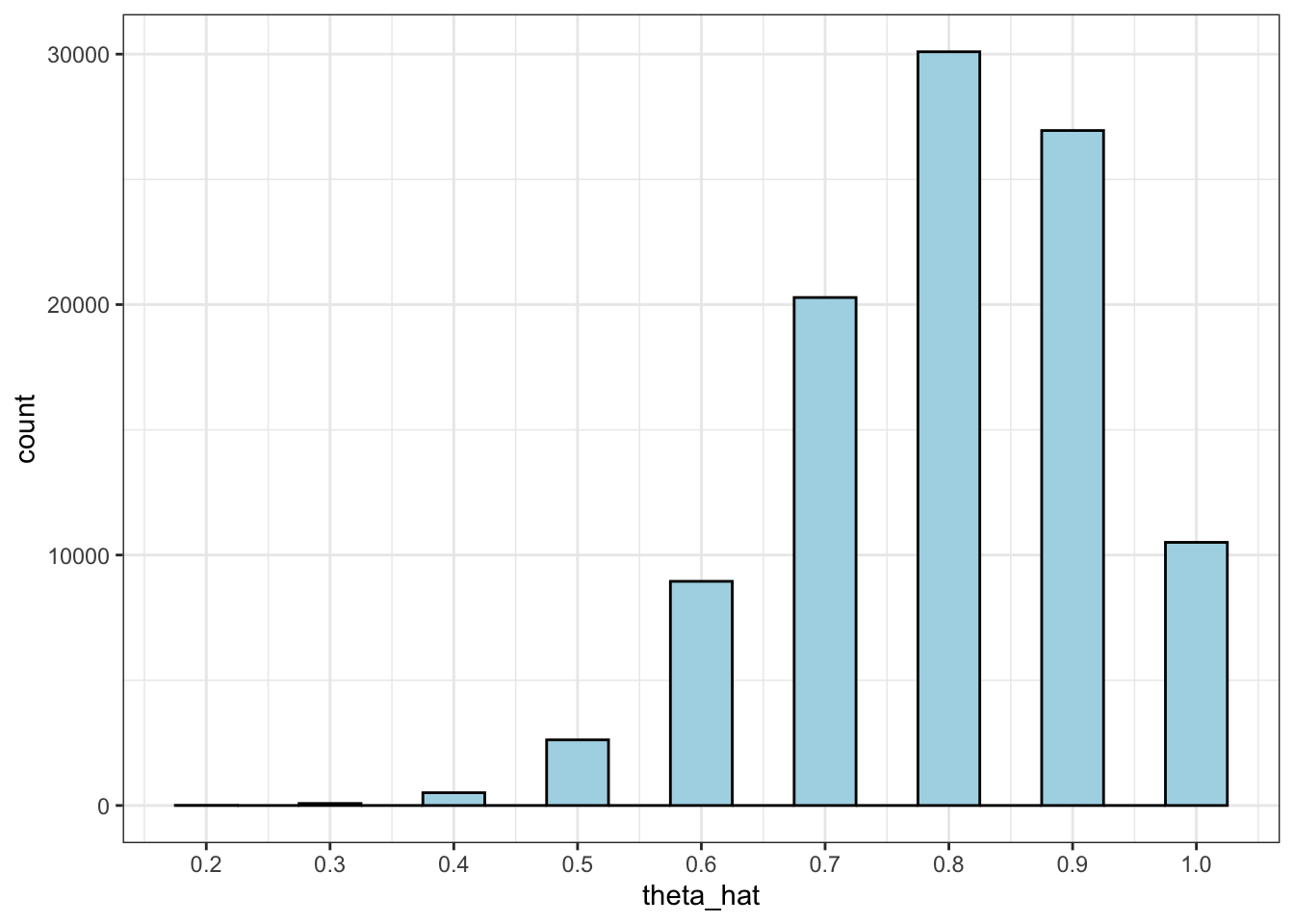
In Figure 1.4 above, it is really evident that under repeated sampling, it is obvious to pick “the best” estimator value \(\hat\theta\), say, by choosing the value corresponding to the highest bar.
But we cannot “do” repeated sampling most of the time. It is too tiresome, expensive, and just not feasible or impossible sometimes! (Think clinical trials… can you repeat the trial 10,000 times?!). Can we still do something about it then? Yes! By studying statistics from a mathematical angle, we can come up with neat results to come up with reliable statements about the variability of estimators.
Estimators (such as \(\hat\theta=\bar X_n\)) are functions of random variables, and therefore are themselves random (i.e. have variability).
Figuring out the distribution of estimators is the central idea around statistics.
From the distribution of \(\hat\theta\), we can know
\usetikzlibrary{fit,positioning,shapes.geometric,decorations.pathreplacing,calc}
\begin{tikzpicture}[scale=0.8, transform shape]
\tikzstyle{obsvar}=[rectangle, thick, minimum size = 10mm,draw =black!80, node distance = 1mm]
\tikzstyle{connect}=[-latex, thick]

\node[obsvar] (fx) [] {$\hspace{1em}f(x|\theta)\hspace{1em}$};
\node (xx) [right=of fx] {\textcolor{blue}{$\{X_1,\dots,X_n\}$}};
\node (theta) [left=of fx] {\textcolor{red}{$\theta$}};
\node (d1) [below=of fx,yshift=9mm] {Model};
\node (d2) [below=of xx,yshift=11mm] {\scriptsize \textcolor{blue}{prob.}};
\node (d3) [below=of theta,yshift=11mm] {\scriptsize \textcolor{red}{param.}};
\node (d1) [above=of fx,yshift=-5mm] {\underline{Probability}};

\path (fx) edge [connect] (xx)
      (theta) edge [connect] (fx);

\end{tikzpicture}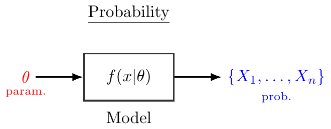
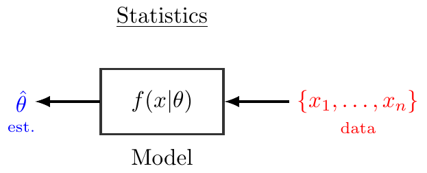
\usetikzlibrary{fit,positioning,shapes.geometric,decorations.pathreplacing,calc}
\begin{tikzpicture}[scale=0.8, transform shape]
\tikzstyle{obsvar}=[rectangle, thick, minimum size = 10mm,draw =black!80, node distance = 1mm]
\tikzstyle{connect}=[-latex, thick]
\node[obsvar] (fx) [] {$\hspace{1em}f(x|\theta)\hspace{1em}$};
\node (xx) [right=of fx] {\textcolor{red}{$\{x_1,\dots,x_n\}$}};
\node (theta) [left=of fx] {\textcolor{blue}{$\hat\theta$}};
\node (d1) [below=of fx,yshift=9mm] {Model};
\node (d2) [below=of xx,yshift=11mm] {\scriptsize \textcolor{red}{data}};
\node (d3) [below=of theta,yshift=11mm] {\scriptsize \textcolor{blue}{est.}};
\node (d1) [above=of fx,yshift=-5mm] {\underline{Statistics}};

\path (fx) edge [connect] (theta)
      (xx) edge [connect] (fx);

\end{tikzpicture}