Example 3.1 Consider the time to failure (in years) for circuit boards modelled by \(\mathop{\mathrm{Exp}}(\lambda)\). An independent random sample \(X_1,\dots,X_n\) was collected. What is the probability that the minimum time lasted is more than 2 years? \[\begin{align*}
\operatorname{P}(\min\{X_1,\dots,X_n\} > 2)
&=\operatorname{P}(X_1 > 2, \dots, X_n > 2) \\
&=\operatorname{P}(X_1>2)\cdots\operatorname{P}(X_n>2)\\
&= \left[\operatorname{P}(X_1 > 2)\right]^n \\
&= [e^{-2/\lambda}]^n \\
&= e^{-2n/\lambda}
\end{align*}\]
A reasonable estimator for \(1/\lambda\) is \(T_n=\min\{X_1,\dots,X_n\}\).
3.2 Finite vs inifinite population
Infinite population
Implicitly iid: “Removing” \(X_1=x_1\) from the population does not affect the probability distribution for the subsequent samples. Why “infinite”? In scenarios where the exact population size is either unknown, uncountable, or effectively limitless, it is simpler to treat it as infinite.
Finite population
Not necessarily iid, depending on the sampling method:
Example 3.2 Estimate the average height of goalkeepers. Which ones? Presumably all of them–past, present, and future–in all leagues. For all intents and purposes, this is an infinite population.
3.3 An experiment
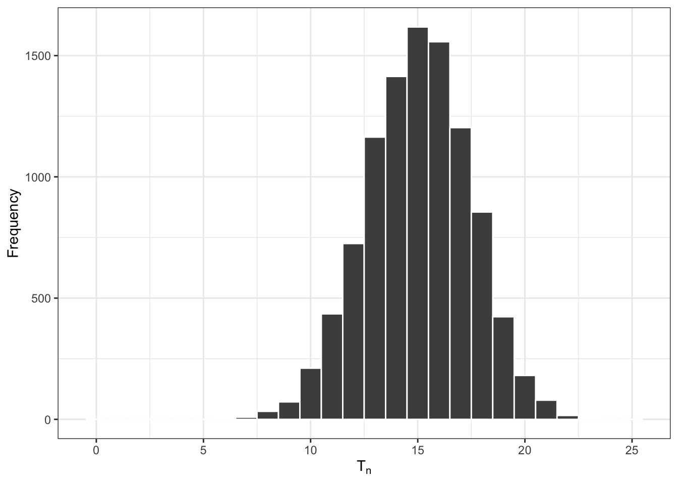
Using R, we can draw multiple instances of the statistic \(T_n\). Let \(n=25\) and \(p=0.6\) (true value).
n <-25p <-0.6B <-10000x <-rbinom(B, n, p)# First 10 valueshead(x, 10)
[1] 19 15 15 14 16 17 20 18 17 17
Code
ggplot() +geom_histogram(aes(x), fill ="gray30", col ="white", breaks =seq(-0.5, n +0.5, by =1)) +scale_x_continuous(breaks =seq(0, n, by =5)) +labs(x =expression(T[n]), y ="Frequency")