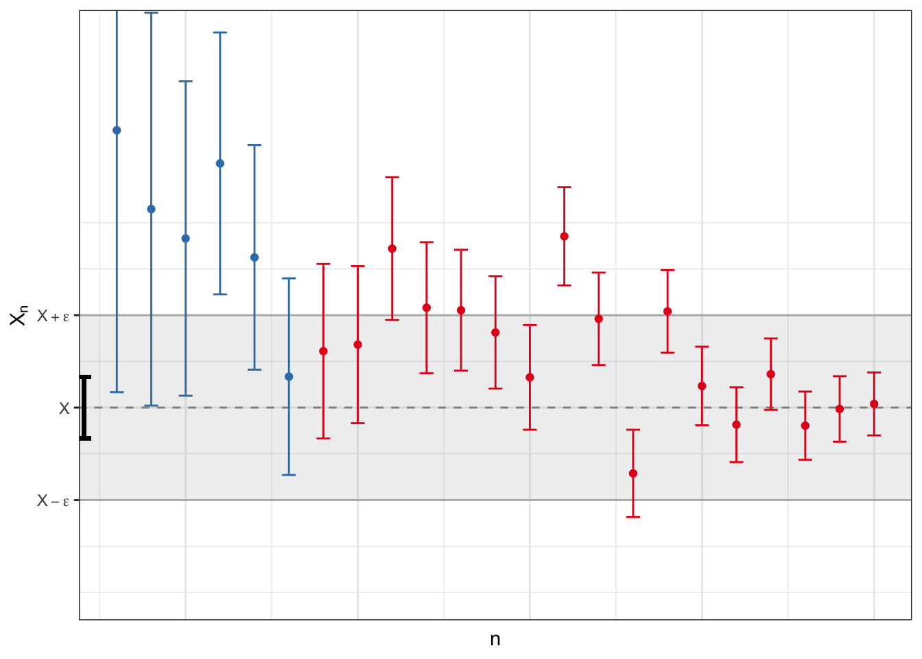
While there is no guarantee that the points will eventually stay inside the \(\epsilon\)-band, the probability of it being outside the band tends to 0.
Definition 4.1 (Almost sure convergence)\(X_n\) converges to \(X\) in almost surely if for every \(\epsilon>0\), \[
\operatorname{P}\left(\lim_{n\to\infty} |X_n-X|\geq\epsilon \right) = 0.
%\ \Leftrightarrow \ \Pr\left(\lim_{n\to\infty} |X_n-X| < \epsilon \right) = 1.
\] We write \(X_n\xrightarrow{\text{a.s.}}X\).
That is, \(X_n(\omega)\to X(\omega)\) for all outcomes \(\omega \in \Omega\), except perhaps for a collection of outcomes \(\omega \in A\) with \(\operatorname{P}(A) = 0\). This is stronger than (i.e. it implies, but is not implied by) convergence in probability. There is no relationship between convergence in mean square and convergence almost surely.
4.3 The Strong Law of Large Numbers
With the same setup as for WLLN, a different argument leads to the stronger conclusion as per the result below.
Theorem 4.1 (Strong Law of Large Numbers) Let \(X_1,X_2,\dots\) be iid rvs with mean \(\mu\) and variance \(\sigma^2\). Let \(\bar X_n\) denote the sample mean, i.e. \[
\bar X_n = \frac{1}{n}\sum_{i=1}^n X_i.
\] Then, \(\bar X_n{\xrightarrow{\text{a.s.}}} \mu\) as \(n\to\infty\), i.e. \[
\operatorname{P}\left(\lim_{n\to\infty} |\bar X_n-\mu| < \epsilon \right) = 1.
\]
Proof is outside the scope of this module. It’s satisfying to know that the SLLN exists, but for our purposes, WLLN suffices!