Code
X <- rnorm(n = 100, mean = 8)
mean(X)
[1] 7.986668Here’s how we simulation \(n=100\) random sample from a normal distribution with mean \(\mu=8\) and \(\sigma=1\).
X <- rnorm(n = 100, mean = 8)
mean(X) [1] 7.986668The mean is found to be 7.99. Here’s a plot of the log-likelihood function (\(\mu\) against \(\ell(\mu)\)):
tibble(
  x = mean(X) + seq(-1, 1, length = 100)
) |>
  rowwise() |>
  mutate(y = sum(dnorm(X, mean = x, log = TRUE))) |>
  ggplot(aes(x, y)) +
  geom_line() +
  geom_segment(linetype = "dashed", x = mean(X), xend = mean(X), y = -Inf,
               yend = sum(dnorm(unlist(X), mean = mean(X), log = TRUE)),
               size = 0.4, col = "gray") +
  labs(x = expression(mu), y = expression(l(mu)))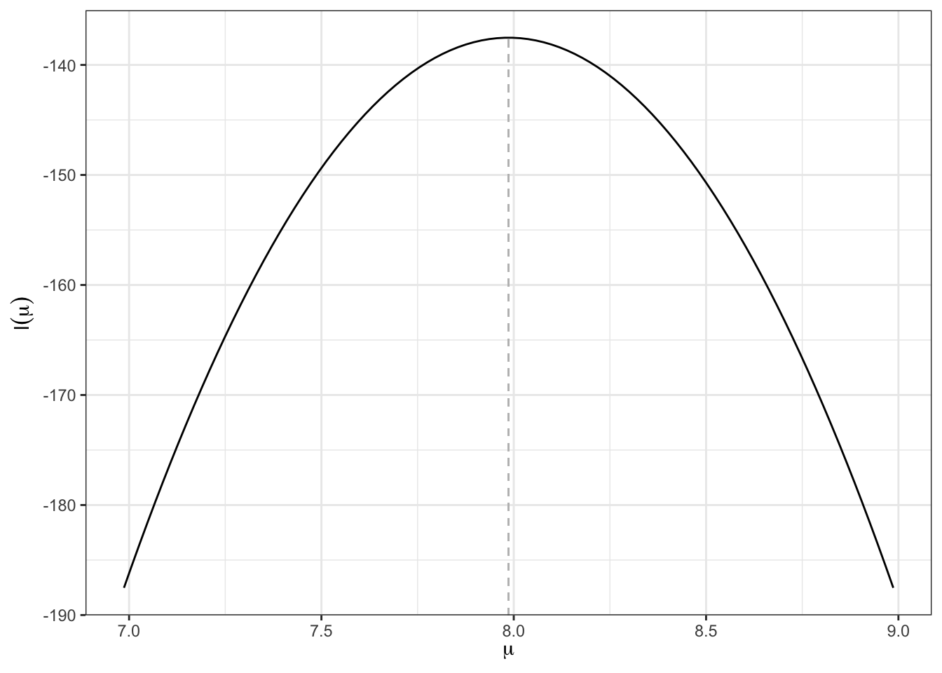
Here’s how to optimise the (log-)likelihood function.
neg_loglik <- function(theta, data = X) {
  -1 * sum(dnorm(x = data, mean = theta, log = TRUE))
}

res <- nlminb(
  start = 1,  # starting value
  objective = neg_loglik,
  control = list(
    trace = 1  # trace the progress of the optimiser
  ))
0: 2578.2008: 1.00000
1: 583.53365: 5.00000
2: 137.52440: 7.98669
3: 137.52440: 7.98667
4: 137.52440: 7.98667glimpse(res)List of 6
$ par : num 7.99
$ objective : num 138
$ convergence: int 0
$ iterations : int 4
$ evaluations: Named int [1:2] 6 7
..- attr(*, "names")= chr [1:2] "function" "gradient"
$ message : chr "relative convergence (4)"It is possible to reduce the variance of an unbiased estimator by conditioning on a sufficient statistic.
Theorem 5.1 (Rao-Blackwell) Suppose that \(\hat\theta({\mathbf X})\) is unbiased for \(\theta\), and \(S({\mathbf X})\) is sufficient for \(\theta\). Then the function of \(S\) defined by \[ \phi(S) = \mathop{\mathrm{E}}_\theta(\hat\theta|S) \]
In other words, \(\phi(S)\) is a uniformly unbiased estimator for \(\theta\). Thus the Rao-Blackwell theorem provides a systematic method of variance reduction for an estimator that is not a function of the sufficient statistic.
Proof.
Since \(S\) is sufficient, the distribution of \({\mathbf X}\) given \(S\) does not involve \(\theta\), and hence \(\mathop{\mathrm{E}}_\theta(\hat\theta({\mathbf X})|S)\) does not involve \(\theta\).
\(\mathop{\mathrm{E}}(\phi(S)) = \mathop{\mathrm{E}}\left[ \mathop{\mathrm{E}}(\hat\theta|S) \right] = \mathop{\mathrm{E}}(\hat\theta) = \theta\).
Using the law of total variance, \[\begin{align*} \mathop{\mathrm{Var}}(\hat\theta) &= \mathop{\mathrm{E}}\left[ \mathop{\mathrm{Var}}(\hat\theta|S) \right] + \mathop{\mathrm{Var}}\left[ \mathop{\mathrm{E}}(\hat\theta|S) \right] \\ &= \mathop{\mathrm{E}}\left[ \mathop{\mathrm{Var}}(\hat\theta|S) \right] + \mathop{\mathrm{Var}}(\phi(S)) \\ &\geq \mathop{\mathrm{Var}}(\phi(S)), \end{align*}\] with equality iff \(\mathop{\mathrm{Var}}(\hat\theta|S) =0\), i.e. iff \(\hat\theta\) is a function of \(S\).
Example 5.1 Suppose we have data \(X_1,\dots,X_n\,\overset{\text{iid}}{\sim}\,\mathop{\mathrm{Poi}}(\lambda)\) pertaining to the number of road accidents per day, and we want to estimate the probability of having no accidents \(\theta = e^{-\lambda}=\operatorname{P}(X_i=0)\).
An unbiased estimator of \(\theta\) is \[ \hat\theta({\mathbf X}) = \begin{cases} 1 & X_1 =0 \\ 0 & \text{otherwise,} \end{cases} \] as \(\mathop{\mathrm{E}}\hat\theta({\mathbf X}) = 1\cdot\operatorname{P}(X_1=0)=e^{-\lambda}=\theta\). But this is likely to be a poor estimator, since it ignores the rest of the sample \(X_2,X_3,\dots,X_n\).
We can see that \(S({\mathbf X})=\sum_{i=1}^n X_i\) is sufficient since the joint pdf can be expressed as \[ f({\mathbf x}|\lambda) = \frac{1}{x_1!\cdots x_n!} \cdot e^{-n\lambda}\lambda^{\sum_{i=1}^nx_i}. \]
Now apply the Rao-Blackwell theorem: \[\begin{align*} \phi(S) = \mathop{\mathrm{E}}(\hat\theta|S) = \mathop{\mathrm{E}}\Big(\hat\theta \, \Big| \, \sum_{i=1}^n X_i = S \Big) &= \operatorname{P}\Big(X_1=0 \, \Big| \, \sum_{i=1}^n X_i = S \Big)\\ &= \left(1 - \frac{1}{n} \right)^S, \end{align*}\] where the conditional probability in the last step comes from the Poisson-binomial relationship (Refer Ex. Sheet 2: Suppose \(X_i\,\overset{\text{iid}}{\sim}\,\mathop{\mathrm{Poi}}(\lambda_i)\), then \(X_1\big|(\sum_{i=1}^nX_i=m)\sim\mathop{\mathrm{Bin}}(m,\pi)\), where \(\pi=\lambda_1/\sum_{i=1}^n \lambda_i\)).
By the Rao-Blackwell theorem, \(\mathop{\mathrm{Var}}(\phi)<\mathop{\mathrm{Var}}(\hat\theta({\mathbf X}))\) (strict inequality since \(\hat\theta({\mathbf X})\) is not a function of \(S\)), so prefer \(\phi(S)\) over \(\hat\theta({\mathbf X})\) as an estimator.
lambda <- 2
n <- 25
(theta <- dpois(x = 0, lambda = lambda))
[1] 0.1353353B <- 1000
X <- matrix(rpois(n * B, lambda = lambda), ncol = B)
theta_hat <- apply(X, 2, function(x) as.numeric(x[1] == 0))
phi_hat <- apply(X, 2, function(x) (1-1/n)^(sum(x)))
tibble(theta_hat, phi_hat) %>%
pivot_longer(everything(), names_to = "Estimator", values_to = "theta_hat") %>%
ggplot() +
geom_density(aes(theta_hat, col = Estimator, fill = Estimator), alpha = 0.6) +
# # geom_vline(xintercept = theta, linetype = "dashed") +
# geom_vline(data = tibble(
# x = c(mean(MLE), mean(MOM)),
# Estimator = c("MLE", "MOM")
# ), aes(xintercept = x), linetype = "dashed") +
facet_grid(. ~ Estimator) +
# labs(x = expression(hat(theta)), y = expression(f~(hat(theta)))) +
# scale_x_continuous(breaks = seq(2, 14, by = 2)) +
theme(legend.position = "none")
# geom_text(data = tibble(x = c(4.9, 5.85), y = c(0.45, 0.45),
# Estimator = c("MLE", "MOM"),
# label = c("E(hat(theta)[ML])", "E(hat(theta)[MOM])")),
# aes(x, y, label = label), parse = TRUE)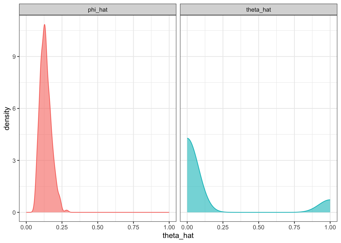
But is \(\phi(S)=(1-1/n)^S\) unbiased? This is guaranteed by the RB theorem. Check: Since \(S=\sum_{i=1}^n X_i \sim\mathop{\mathrm{Poi}}(n\lambda)\), we get \[\begin{align*} \mathop{\mathrm{E}}(\phi(S)) &= \sum_{s=0}^\infty \left(1 - \frac{1}{n} \right)^s \frac{e^{-n\lambda}(n\lambda)^s}{s!}\times e^{-\lambda}e^{\lambda} \\ &= e^{-\lambda} \sum_{s=0}^\infty {\color{gray}\underbrace{\color{black}\frac{e^{-\lambda(n-1)}[\lambda(n-1)]^s}{s!}}_{\text{pmf of }\mathop{\mathrm{Poi}}(\lambda(n-1))}} = e^{-\lambda}. \end{align*}\] A similar calculation can give us the variance of this estimator.
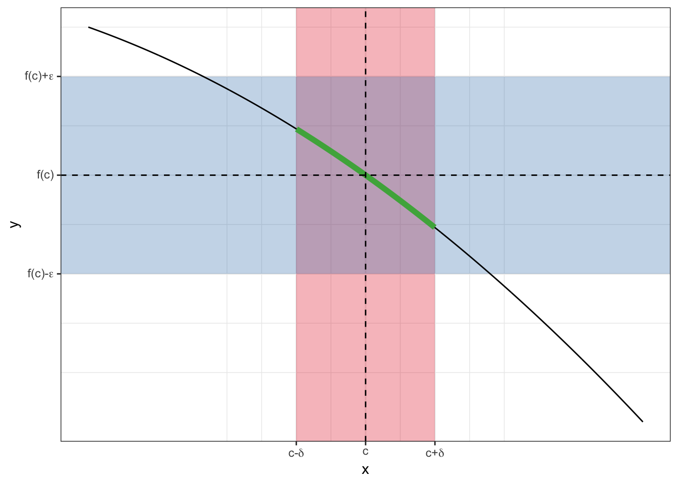
A continuous function \(\psi(x)\) is a function such that a continuous variation of \(x\) induces a continuous variation of \(\psi(x)\)–i.e. no jumps allowed.
tibble(
  x = seq(1, 3, length = 1000),
  y = 16 - x^2
) -> plot_df

mycols <- grDevices::palette.colors(3, palette = "Set1")

ggplot() +
  annotate("rect", xmin = 2 - 0.25, xmax = 2 + 0.25, ymin = -Inf, ymax = Inf,
           fill = mycols[1], alpha = 0.3) +
  annotate("rect", xmin = -Inf, xmax = Inf, ymin = 12 - 2, ymax = 12 + 2,
           fill = mycols[2], alpha = 0.3)  +
  geom_line(data = plot_df, aes(x, y)) +
  geom_line(data = plot_df %>% filter(x >= 2 - 0.25, x <= 2 + 0.25), aes(x, y),
            col = mycols[3], linewidth = 2) +
  # geom_segment(aes(x = 2, xend = 2, y = 12, yend = -Inf), linetype = "dashed",
  #              size = 0.4)
  geom_hline(yintercept = 12, linetype = "dashed") +
  geom_vline(xintercept = 2, linetype = "dashed") +
  scale_x_continuous(breaks = 2 + c(-0.25, 0, 0.25),
                     labels = c(expression("c-"*delta),
                                "c",
                                expression("c+"*delta))) +
  scale_y_continuous(breaks = 12 + c(-2, 0, 2),
                     labels = c(expression("f(c)-"*epsilon),
                                "f(c)",
                                expression("f(c)+"*epsilon)))