2  Commonly used probability models

2.1 Poisson-Binomial relationship

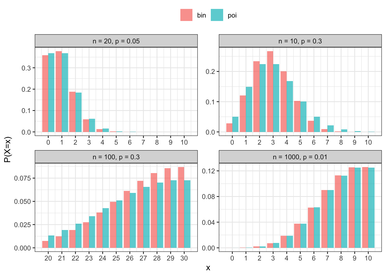
The Poisson distribution plays a useful approximation role for the binomial: \[ X\sim\mathop{\mathrm{Bin}}(n,p) \ \ \Rightarrow \ \ X \approx \mathop{\mathrm{Poi}}(np) \] when \(n\) is large (\(n>20\)) and \(np\) is small (\(np<5\)). The reason is the Poisson can be seen as the limiting case to the binomial as \(n\to\infty\) while \(\mathop{\mathrm{E}}(X)=np\) remains fixed.

\[\begin{align*} \lim_{n\to\infty} \operatorname{P}(X=x) &= \lim_{n\to\infty} \frac{n!}{x!(n-x)!}\left(\frac{\lambda}{n} \right)^x \left(1 - \frac{\lambda}{n} \right)^{n-x} \\ &= \frac{\lambda^x}{x!} \lim_{n\to\infty} {\color{gray}\underbrace{\color{black}\frac{n!}{n^x(n-x)!}}_{\to 1}} \, {\color{gray}\underbrace{\color{black}\left(1 - \frac{\lambda}{n} \right)^n}_{\to e^{-\lambda}}} \, {\color{gray}\underbrace{\color{black}\left(1 - \frac{\lambda}{n} \right)^{-x}}_{\to 1}} \\ &= \frac{e^{-\lambda}\lambda^x}{x!} \\ &= \operatorname{P}(Y=x), Y\sim\mathop{\mathrm{Poi}}(\lambda). \end{align*}\]

The reason is that the Poisson can be seen as the limiting case to the binomial as \(n\to\infty\) while \(\mathop{\mathrm{E}}(X)=np\) remains fixed.

library(tidyverse)
poibin_df <- function(n, p, x = 0:10) {
  lambda <- n * p
  the_title <- paste0("n = ", n, ", p = ", p)
  
  tibble(
    x = x,
    bin = dbinom(x, size = n, prob = p),
    poi = dpois(x, lambda = n * p)
  ) %>%
    pivot_longer(-x) %>%
    mutate(title = the_title)
}

plot_df <- bind_rows(
  poibin_df(20, 0.05),
  poibin_df(10, 0.3),
  poibin_df(100, 0.3, 20:30),
  poibin_df(1000, 0.01)
) 
mylevels <- unique(plot_df$title)
plot_df$title <- factor(plot_df$title, levels = mylevels)
# levels(plot_df$title) <- mylevels
  
ggplot(plot_df, aes(x, value, fill = name)) +
  geom_bar(stat = "identity", position = "dodge", alpha = 0.7) +
  facet_wrap(. ~ title, ncol = 2, scales = "free") +
  scale_x_continuous(breaks = 0:100) +
  # scale_fill_manual(values = c(palgreen, palred)) +
  labs(y = "P(X=x)", col = NULL, fill = NULL) +
  theme(legend.position = "top")

Figure 2.1

2.2 Memoryless property

\(X\) is a positive rv and memoryless, in the sense that for all \(t>s>0\), \[ \operatorname{P}(X > t+s \mid X>s) = \operatorname{P}(X > t) \] if and only if it is exponentially distributed¹.

Given that we have been waiting for \(s\) units of time, the probability that we wait a further \(t\) units of time is independent to the first fact!

Example 2.1 Assume that bus waiting times are exponentially distributed, and you are concerned about the event \(A=\) a bus arrives in the next minute. Let \(p_i = \operatorname{P}(A|B_i)\) where

1. \(B_1 =\) you just arrived to the station; and
2. \(B_2 =\) you’ve been sitting there for 20 minutes already.

Then \(p_1=p_2\).

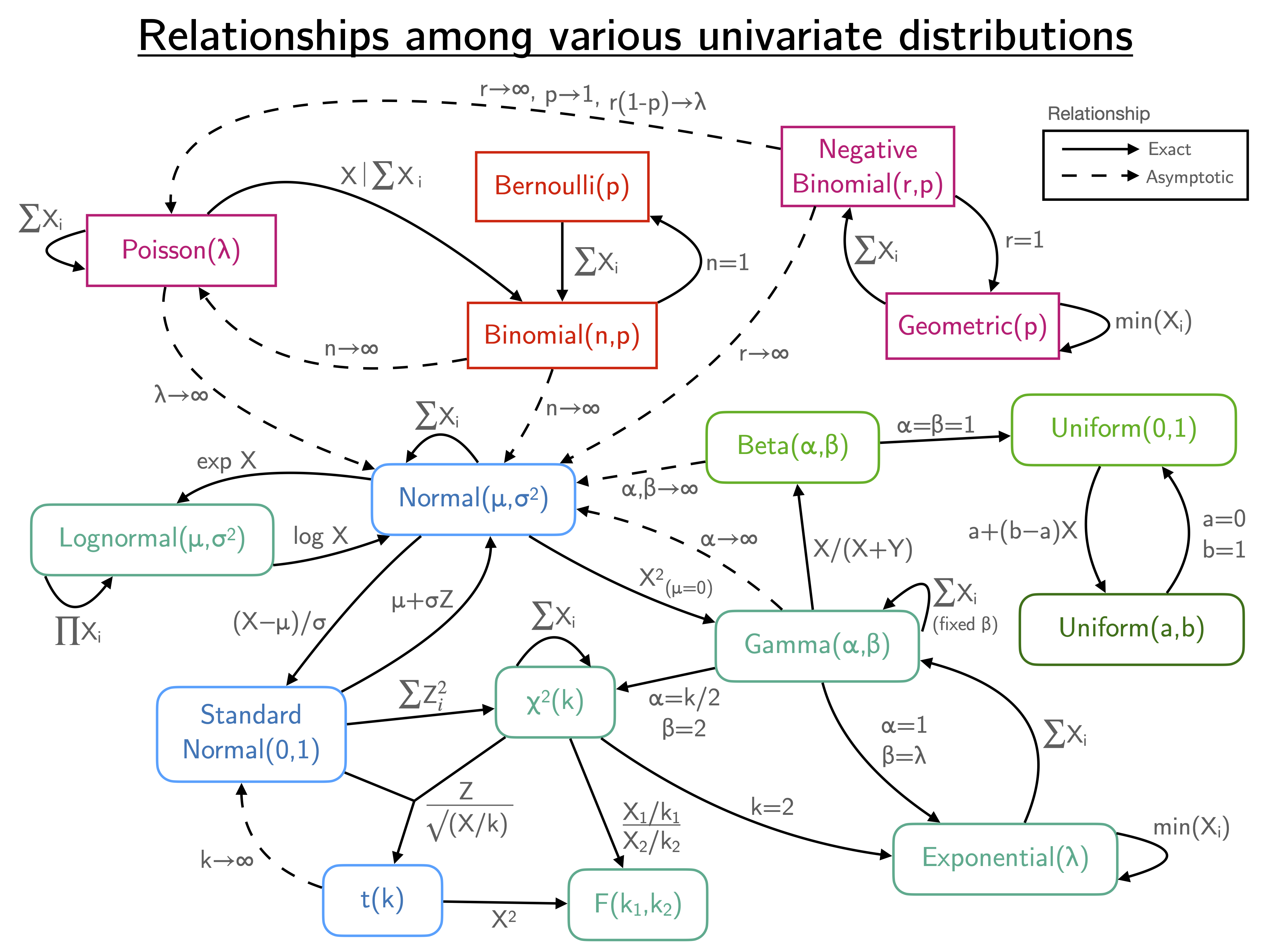
2.3 Relationships

Figure 2.2: Relationships among various univariate distributions.

---

1. https://perplex.city/memorylessness-at-the-bus-stop-f2c97c59e420?gi=3602158da66b