8 Using `nlminb()` for Maximum Likelihood Estimation

Modified

April 9, 2025

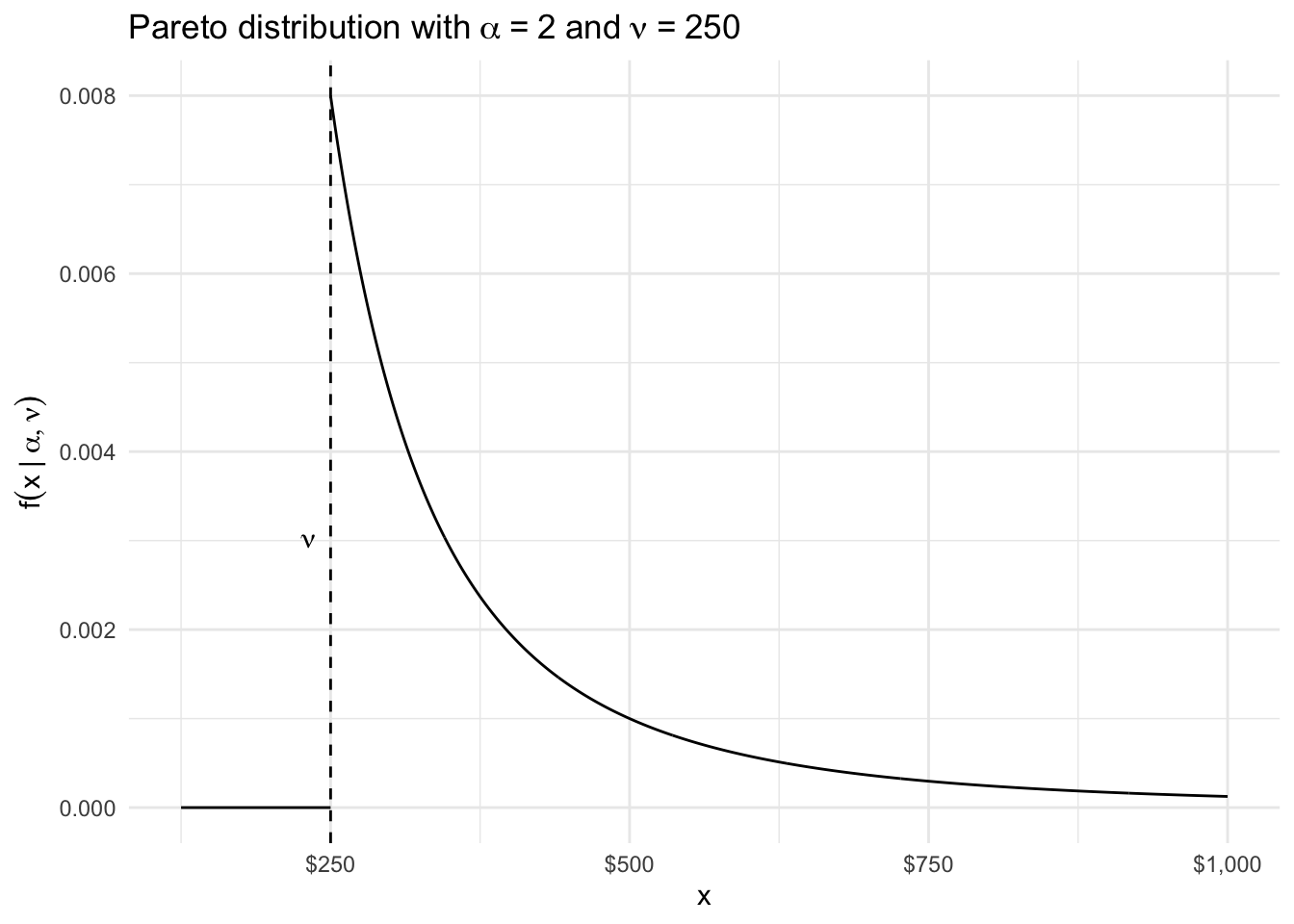
Consider Q2 in the Exercise Sheet 5 (Hypothesis Testing). A random sample $X_1,\dots,X_n$ is drawn from a Pareto distribution with pdf \[ f(x \mid \alpha,\nu) = \frac{\alpha\nu^\alpha}{x^{\alpha+1}} \quad \text{for } x > \nu, \ \alpha > 0, \ \nu > 0 \] The Pareto distribution is frequently used in economics to model income and wealth distributions, especially the upper tail–where a small fraction of the population holds a disproportionately large share of income or wealth. This fits the famous Pareto Principle or 80/20 rule.

The two parameters in the Pareto distribution:

$\nu$ (scale parameter): the minimum possible income/wealth (i.e., the distribution starts at this value),
$\alpha$ (shape parameter): controls the “fatness” of the tail, smaller $\alpha$ means fatter tails and greater inequality. In wealth modelling, this is the so-called Pareto index.

An example from empirical literature (e.g. Atkinson and Piketty, 2007) suggests that $\alpha$ for income in the U.S. top 1% is around 1.5-2.5, depending on the year and method, while $\nu$ varies depending on the income bracket analyzed, typically $100k to $500k for high earners.

Here is what the pdf looks like:

Code

# True values
alpha <- 2  # shape parameter
nu <- 250  # thousands of dollars, say

tibble(
  x = seq(nu, nu*4, length.out = 1000),
  f = case_when(
    x < alpha ~ 0,
    TRUE ~ alpha * nu^alpha / x^(alpha + 1)
)) |>
  ggplot(aes(x, f)) +
  geom_line() +
  geom_vline(xintercept = nu, linetype = "dashed") +
  annotate("segment", x = nu, xend = nu / 2, y = 0, yend = 0) +
  annotate("text", x = nu, y = 3e-3, label = expression(nu), hjust = 2) +
  labs(
    title = expression("Pareto distribution with"~alpha~"="~2~"and"~nu~"="~250),
    x = "x",
    y = expression(f(x~"|"~alpha, nu))
  ) +
  scale_x_continuous(labels = scales::dollar) +
  theme_minimal()

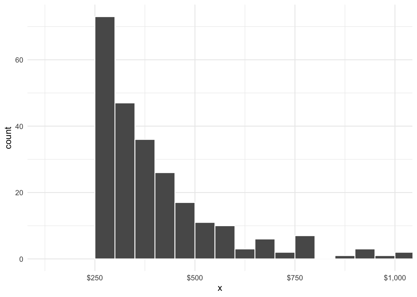
The following code generates a random sample of size $n$ from the Pareto distribution with parameters $\alpha = 2$ and $\nu = 250$:

Code

library(VGAM)
set.seed(1)

n <- 250  # sample size
X <- rpareto(n, scale = nu, shape = alpha)
head(X, 10)

 [1]  485.1775  409.8229  330.3074  262.3297  556.6811  263.7592  257.2164
 [8]  307.5429  315.1921 1005.7592

Code

summary(X)

   Min. 1st Qu.  Median    Mean 3rd Qu.    Max. 
  250.9   292.4   354.7   428.1   469.4  2186.1

And suppose we were to plot a histogram of the sample:

Code

ggplot(data.frame(x = X), aes(x)) +
  geom_histogram(col = "white", binwidth = 50, boundary = nu) +
  scale_x_continuous(labels = scales::dollar) +
  coord_cartesian(xlim = c(nu / 2, 1000)) +
  theme_minimal()

Think

When we “draw” samples from a particular pdf, we expect the distribution of the sample (i.e., the histogram) to resemble the theoretical pdf. Do you see any resemblance? Looking ahead to parameter estimation, suppose the true value of $\nu$ was not known. What value would you guess for $\nu$ based on the data?

8.1 Paremeter estimation using MLE

In class, we solved for the MLE of $\alpha$ and $\nu$ in the usual way using derivatives and sketching the likelihood function. Recall that \[ \hat\alpha = \frac{n}{\sum_{i=1}^n \log(X_i/\hat\nu)} \quad \text{and} \quad \hat\nu = \min(X_i). \]

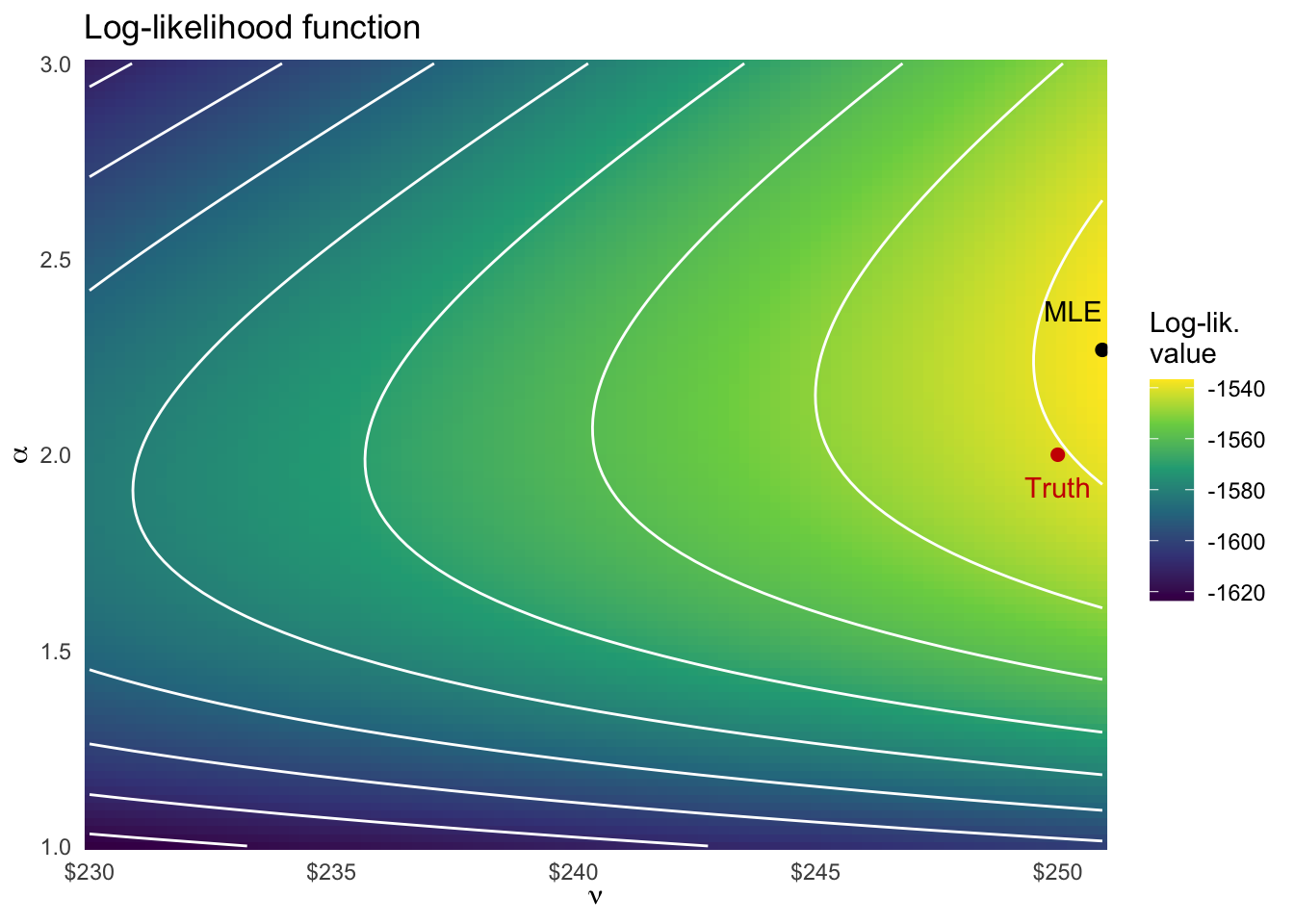
If we plug in the data to compute the MLE, we get:

Code

nu_hat <- min(X)
alpha_hat <- n / sum(log(X / nu_hat))
cat("nu_hat =", nu_hat, "\nalpha_hat =", alpha_hat)

nu_hat = 250.9195 
alpha_hat = 2.267916

We can also let the computer do the work for us using the nlminb() function in R. This function is a general-purpose optimization function that can be used to find the maximum likelihood estimates of parameters in a statistical model. What we need is to first code the likelihood function, and then use nlminb() to find the values of $\alpha$ and $\nu$ that maximize the likelihood function.

Code

# The pdf function
fx <- function(x, alpha, nu) {
  alpha * nu^alpha / x^(alpha + 1)
}
fx(X[1:10], alpha, nu)

 [1] 0.0010944805 0.0018160229 0.0034686077 0.0069241716 0.0007245869
 [6] 0.0068121958 0.0073453722 0.0042972722 0.0039919405 0.0001228649

Code

# The log-likelihood function
ll <- function(theta) {
  alpha <- theta[1]
  nu <- theta[2]
  
  # Return really small value if support condition is violated
  if (alpha <= 0 | nu <= 0 | any(X < nu)) return(-1e10)
  
  sum(log(fx(X, alpha, nu)))
}
ll(theta = c(2, 250))

[1] -1540.532

Here’s a plot of the 2-dimensional log-likelihood function based on the data:

Code

expand_grid(
  nu = seq(230, min(X), length.out = 100),
  alpha = seq(1, 3, length.out = 100)
) |>
  mutate(ll = purrr::map2_dbl(alpha, nu, ~ll(c(.x, .y)))) |>
  filter(ll > -1e10) |>
  ggplot(aes(nu, alpha, z = ll)) +
  geom_raster(aes(fill = ll)) +
  geom_contour(color = "white") +
  scale_fill_viridis_c() +
  annotate("point", x = nu, y = alpha, color = "red3", size = 2) +
  annotate("text", x = nu, y = alpha + 0.1, label = "Truth", color = "red3", vjust = 4) +
  annotate("point", x = nu_hat, y = alpha_hat, size = 2) +
  annotate("text", x = nu_hat, y = alpha_hat + 0.1, label = "MLE", vjust = 0.5, hjust = 1) +
  scale_x_continuous(labels = scales::dollar, expand = c(0, 0)) +
  scale_y_continuous(expand = c(0, 0)) +
  labs(
    title = "Log-likelihood function",
    x = expression(nu),
    y = expression(alpha),
    fill = "Log-lik.\nvalue"
  ) +
  theme_minimal()

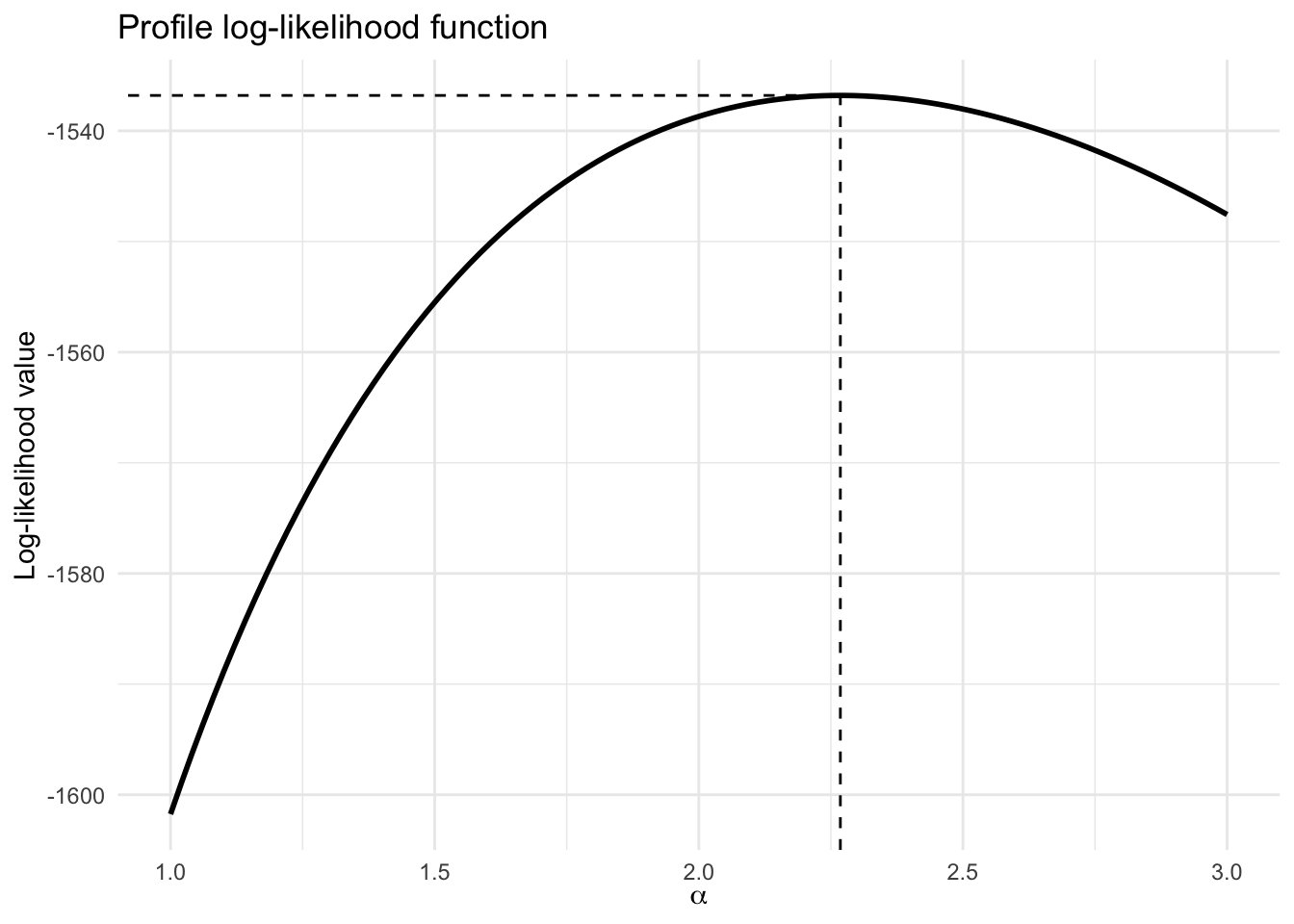
The profile log-likelihood function \[ f(\alpha) = \max_{\nu} \ell(\alpha, \nu) = \ell(\alpha \mid \hat\nu) \] can be sketched as follows:

Code

tibble(
  alpha = seq(1, 3, length.out = 100),
  ll = map_dbl(alpha, ~ll(c(.x, nu_hat)))
) |>
  ggplot(aes(alpha, ll)) +
  geom_line(linewidth = 1) +
  geom_segment(
    data = tibble(
      x = c(alpha_hat, alpha_hat),
      y = c(-Inf, ll(c(alpha_hat, nu_hat))),
      xend = c(alpha_hat, -Inf),
      yend = rep(ll(c(alpha_hat, nu_hat)), 2)
    ),
    aes(x = x, y = y, xend = xend, yend = yend),
    linetype = "dashed",
  ) +
  
  theme_minimal() +
  labs(
    title = "Profile log-likelihood function",
    x = expression(alpha),
    y = "Log-likelihood value"
  )

Now, we use nlminb() to find the MLE of $\alpha$ and $\nu$.

Code

res <- nlminb(
  start = c(alpha, nu),  # initial "guess"
  objective = function(theta) -1 * ll(theta),  # negative log-likelihood
  lower = 0,
  upper = c(Inf, min(X))
)
print(res)

$par
[1]   2.267916 250.919541

$objective
[1] 1536.801

$convergence
[1] 0

$iterations
[1] 6

$evaluations
function gradient 
       9       16 

$message
[1] "both X-convergence and relative convergence (5)"

Code

# Compare nlminb to direct calculations. They are identical!
cat("nu_hat (calculation) =", nu_hat, "vs. nu_hat (MLE) =", res$par[2],  
    "\nalpha_hat (calculation) =", alpha_hat, "vs. alpha_hat (MLE) =", res$par[1], "\n")

nu_hat (calculation) = 250.9195 vs. nu_hat (MLE) = 250.9195 
alpha_hat (calculation) = 2.267916 vs. alpha_hat (MLE) = 2.267916

We can also check that the gradients are close to zero at the MLE. But only for the $\alpha$ parameter, since the log-likelihood is not differentiable at $\nu$!

Code

# Gradient at MLE
numDeriv::grad(
  function(theta) -1 * ll(theta), 
  res$par
)

[1] 1.654437e-06 1.937072e+12

The Hessian (observed Fisher information matrix) can also be obtained as follows:

Code

J <- -1 * numDeriv::hessian(ll, res$par)
print(J)

           [,1]          [,2]
[1,] 48.6055593 -6.093646e-01
[2,] -0.6093646  1.350050e+09

Code

solve(J)  # To get asymptotic variance

             [,1]         [,2]
[1,] 2.057378e-02 9.286271e-12
[2,] 9.286271e-12 7.407132e-10

Code

# Standard errors
se <- sqrt(diag(solve(J)))
print(se)

[1] 1.434356e-01 2.721605e-05