On a farm there are 499 white bunnies, and 1 brown bunny. One of the bunnies ravaged through the carrot farm, leaving the farmer furious.
Figure 6.1
Question
Can we say that we know, or reasonably believe with confidence, that it was a white bunny that caused the problem? What’s your proof?1
Assume colour difference is not associated with behavioural differences in rabbits. If we believe that a white rabbit indeed was at fault, the error rate is 1/500 = 0.2%.
Suppose there was a witness that claimed the brown rabbit did it. The witness performed a colour identification test, reporting the right colour 95% of the time. Given the evidence, the probability that a brown rabbit was at fault is
The \(p\)-value is interpreted as a continuous measure of evidence some null hypothesis–there is no point at which the results become ‘significant’.
Remark
Statistical evidence differs from direct evidence (e.g. having CCTV recording in the house). We may never know what exactly happened. The best we can do is to base decisions based on the likelihood of the evidence materialising.
Since \(p({\mathbf X})\) is a statistic, it is a rv. What is its distribution?
Theorem 6.1 (Uniformity of \(p\)-values) If \(\theta_0\) is a point null hypothesis for the parameter of continuous \({\mathbf X}\), then a correctly calculated \(p\)-value \(p_T({\mathbf X})\) based on any test statistic \(W\), is such that \[
p_T({\mathbf X}) \sim \mathop{\mathrm{Unif}}(0,1)
\] in repeated sampling under \(H_0\).
Proof. This is a consequence of the : Suppose that a continuous rv \(T\) has cdf \(F_T(t), \forall t\). Then the rv \(Y=F_T(T)\sim\mathop{\mathrm{Unif}}(0,1)\) because: \[
F_Y(y)=\operatorname{P}( {\color{gray}\overbrace{\color{black}F_T(T)}^{Y}}\leq y) = \operatorname{P}\big(T \leq F^{-1}_T(y)\big) = F_T\left(F^{-1}_T(y) \right) = y,
\] which is the cdf of a \(\mathop{\mathrm{Unif}}(0,1)\) distribution.
Now for any data \({\mathbf x}\), \[
p_T({\mathbf x}) = \operatorname{P}\!{}_{\theta_0}\left(T({\mathbf X}) \geq T({\mathbf x}) \right) = 1 - F\big( T({\mathbf x}) \big),
\] where \(F\) is the cdf (under \(H_0\)) of \(T({\mathbf X})\). Hence, \(p_T({\mathbf x})=1-Y\) where \(Y\sim\mathop{\mathrm{Unif}}(0,1)\) by the probability integral transform. But clearly if \(Y\sim\mathop{\mathrm{Unif}}(0,1)\), then so is \(1-Y\).
This result is useful especially for checking the validity of a complicated \(p\)-value calculation:
Simulate several new data sets from the null distribution.
For each simulated data set, apply the \(p\)-value calculation.
Assess the collection of resulting \(p\)-values–do they seem to be uniformly distributed?
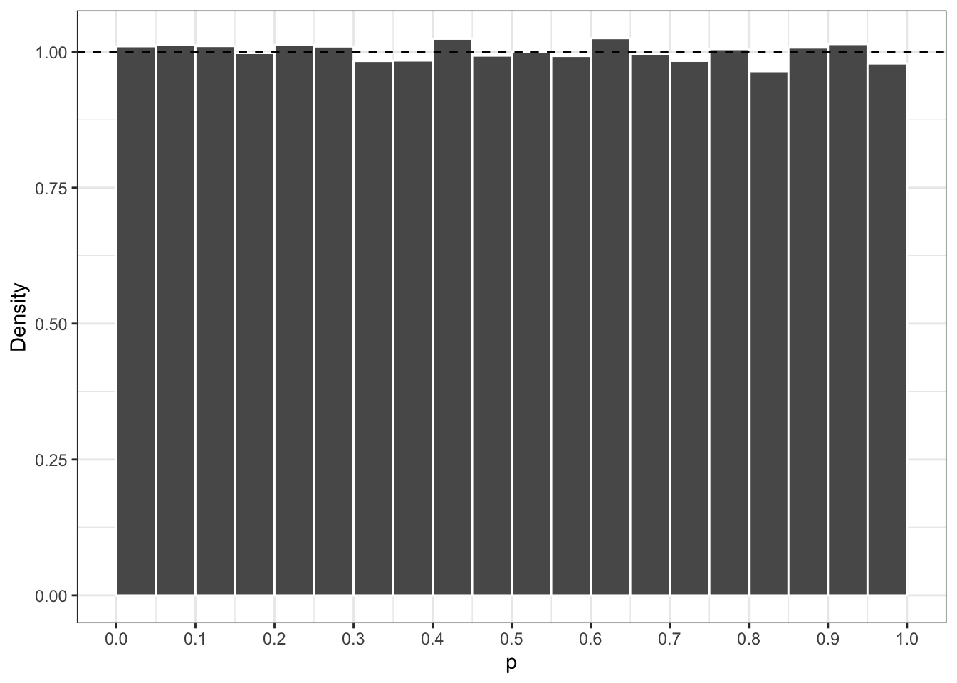
Suppose we are testing \(H_0:\mu=0\) on a random sample of \(X_1,\dots,X_n\) assumed to be normally distributed with mean \(\mu\) and variance \(\sigma^2=4.3^2\). Let’s do this experiment:
Draw \(X_1,\dots,X_{10}\,\overset{\text{iid}}{\sim}\,\mathop{\mathrm{N}}(0,4.3^2)\) (the distribution under \(H_0\))
Compute the \(p\)-value \(p({\mathbf x})\) based on the simulated data
Repeat 1–2 a total of \(B=100000\) times to get \(p_1,\dots,p_B \in (0,1)\)
Plotting a histogram of the simulated \(p\)-values yields:
Code
n <-10sigma <-4.3B <-100000res <-rep(NA, B)for (i in1:B) { x <-rnorm(n, sd = sigma) res[i] <-2* (pnorm((sqrt(n) *abs(mean(x)) / sigma), lower.tail =FALSE))}ggplot() +geom_histogram(aes(res, ..density..), breaks =seq(0, 1, by =0.05),col ="white") +geom_hline(yintercept =1, linetype ="dashed") +scale_y_continuous(breaks =seq(0, 1, by =0.25)) +scale_x_continuous(breaks =seq(0, 1, by =0.1)) +labs(x ="p", y ="Density")
Figure 6.3
Why is this? Assume that \(H_0\) is true. In the Neyman-Pearson approach, \(\alpha\) is the rate of false positives, i.e. the rate at which the null hypothesis is rejected given that \(H_0\) is true. This rate is fixed. On the other hand, \(p=p({\mathbf X})\) is a random variable.
For any value \(\alpha\), the null is rejected when the observed \(p < \alpha\). This happens, by definition, with probability \(\alpha\)! The only way that this happens is when the \(p\)-value comes from a uniform distribution, since \(\operatorname{P}(U \leq u) = u\). I.e., under the null
\(p\) has a 5% chance of being less than \(\alpha=0.05\);
\(p\) has a 10% chance of being less than \(\alpha=0.1\);
etc.
So, as a consequence, if \(H_0\) is false, then (hopefully) the \(p\)-values are biased towards 0.
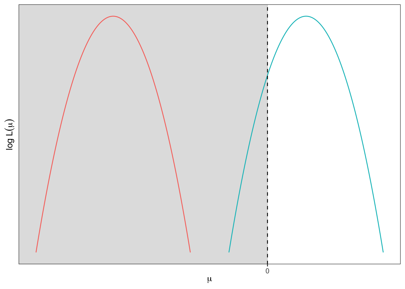
All of the tests thus far are called two-sided tests. Sometimes we wish to measure the evidence (against \(H_0\)) in one direction only.
Example 6.1 Suppose \(X_1,\dots,X_n\,\overset{\text{iid}}{\sim}\,\mathop{\mathrm{N}}(\mu,\sigma^2)\) with \(\sigma^2\) known. Consider testing \(H_0: \mu \leq 0\). The unrestricted MLE remains \(\hat\mu = \bar X\), but the restricted MLE under \(H_0\) is a bit tricky. With a little bit of reasoning, \[
\tilde\mu=\begin{cases}
\bar X & \bar X \leq 0 \\
0 & \bar X > 0
\end{cases}
\]
Therefore, the log LR statistic depends on the value of \(\bar X\): \[
\log W_{LR} = \ell(\hat\mu|{\mathbf X}) - \ell(\tilde \mu|{\mathbf X}) = \begin{cases}
0 & \bar X \leq 0 \\
\frac{n\bar X^2}{2\sigma^2} & \bar X > 0
\end{cases}
\] (the second case when \(\bar X>0\) is as before). The \(p\)-value from data \({\mathbf x}\), using the monotonicity of \(\bar X\) in the LRT statistic, is \[
p({\mathbf x}) = \begin{cases}
1 &\bar x \leq 0 \\
\operatorname{P}(\bar X > \bar x) = 1-\Phi(\sqrt n \bar x / \sigma) &\bar x > 0
\end{cases}
\] Hence, relative to the ‘two-sided’ test that we saw previously, the \(p\)-value is halved if \(\bar x > 0\), and ignores the precise value of \(\bar x\) if \(\bar x \leq 0\).
Further remarks:
Performing a one-sided test instead of a two-sided test thus makes any apparent evidence against \(H_0\) seem stronger (since the \(p\)-value is halved).
In practice there are rather few situations where performing a one-sided test, which assumes that we know in advance that departures from \(H_0\) are in one direction only, can be justified. When assessing the effect of a new drug, for example, the convention is to assess evidence for an effect in either direction, positive or negative.
The two-sided test is said to be more conservative than the one-sided test: The one-sided test risks over-stating the strength of evidence against \(H_0\) if the underlying assumption–that evidence against \(H_0\) counts in one direction only–is actually false.
6.5 “Failing to reject the null hypothesis”
Absence of proof is not proof of absence. You are not able prove a negative.
Australian Tree Lobsters were assumed to be extinct. There was no evidence that any were still living because no one had seen them for decades. Yet in 1960, scientists observed them.
In criminal trial, we start with the assumption that the defendant is innocent until proven guilty. If the prosecutor fails to meet a an evidentiary standard, it does not mean the defendant is innocent.
Accepting the null hypothesis
Accepting the null hypothesis indicates that you have proven that an effect does not exist. Maybe, this is what you mean?2
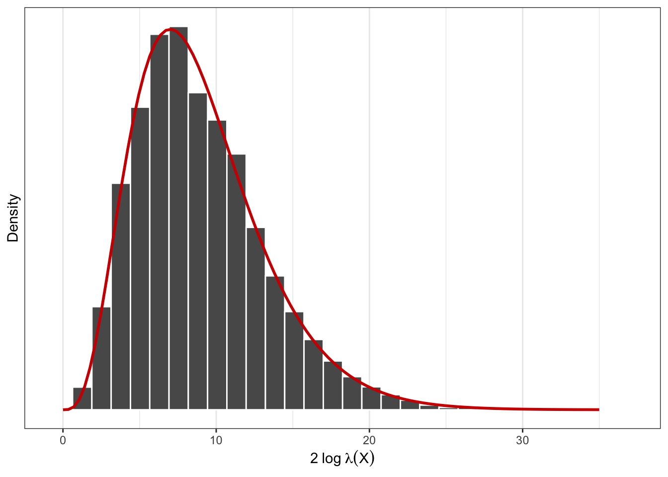
6.6 Asymptotic distribution of LRT: An experiment
Let’s try to “verify” the distribution of the test statistic \(2\log \lambda({\mathbf X})\).
Repeat steps 1–2 \(B=10000\) number of times to get \(T_1,\dots,T_B\)
We can plot the histogram of the observed test statistic, and overlay a \(\chi_9^2\) density over it. As can be seen, it is a good fit.
Code
B <-10000res <-rep(NA, B)for (i in1:B) { X <-rnorm(10, mean =8) res[i] <-sum((X -mean(X)) ^2)}ggplot() +geom_histogram(aes(x = res, y = ..density..), col ="white") +geom_line(data =tibble(x =seq(0, 35, length =100),y =dchisq(x, 10-1)),aes(x, y), col ="red3", size =1) +scale_y_continuous(breaks =NULL) +labs(x =expression(2~log~lambda(X)), y ="Density")
Figure 6.5
Actually, in this particular case, the distribution of \(2\log\lambda({\mathbf X})\) is exact. Note that \[
2 \log \lambda({\mathbf X}) = \frac{n-1}{n-1} \sum_{i=1}^n (X_i-\bar X)^2 = (n-1)S^2
\] which is the sample variance. We’ve seen previously that \[
\frac{(n-1)S^2}{\sigma^2} \sim\chi^2_{n-1}.
\] Thus, \(2\log \lambda({\mathbf X})\) is merely a scaled\(\chi^2\) distribution (but in this case \(\sigma^2=1\)).
Example adapted from Schoeman, F. (1987). Statistical vs. direct evidence. Noûs, 179-198.↩︎